2D N-Body Thermodynamics Simulation
A group project for the NTHU Computational Physics course, using a 2D particle simulation to study ideal-gas behavior, moving-wall compression, and mixing of two particle populations. I built the main structure and first usable version of the simulation code. The final group project added pressure measurements, a spatial grid, inter-particle interactions, and comparisons with thermodynamic predictions.
- ▪Personal contribution: Built the main structure and first usable version of the simulation code.
- ▪Group implementation: Developed a 5×5 spatial partition, moving-wall boundary reflections, pressure output, RK2 time stepping, and collision and repulsive-force models.
- ▪Group analysis: Compared simulated pressure with ideal-gas and adiabatic predictions, and examined particle trajectories, kinetic energy, and mixing.
Methodology
Spatial partition and interactions
The final code partitions the simulation box into a 5×5 grid. Its grid_N.py lookup restricts candidate interactions to nearby cells. Optional short-range repulsion and a simplified equal-mass collision rule are calculated in Numba-compiled loops. The code advances particle positions with an RK2 time-stepping routine.
Boundaries and pressure
The bound_reflection() routine updates four walls, reflects particles that cross them, and adjusts their normal velocity for wall motion. It estimates pressure from the particles' momentum changes over the time step and wall length. Moving one wall provides a compression experiment.
Comparisons
The final report compares simulated pressure with kinetic-theory and two-dimensional adiabatic predictions. It also plots particle trajectories, total kinetic energy, and the velocities of two populations with different initial conditions.
Results & Analysis
Ideal gas and compression
The group report found the general pressure trend but also a substantial discrepancy in the ideal-gas comparison. For moving-wall compression, the simulation agreed most closely with the theoretical curve at the slowest tested boundary speed, 2.5 code units; the deviation grew at higher speeds.
Particle interactions and mixing
The trajectory plots show how adding inter-particle collisions and repulsion changes particle paths. In the mixing experiment, total kinetic energy stayed approximately level, and the two groups' average-speed curves approached one another after about 15 time units.
Figures
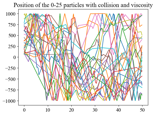
Figure 1: Particle trajectories (0–25) with inter-particle collisions and short-range repulsion — showing their combined effect
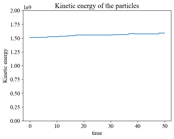
Figure 2: Total kinetic energy vs time — the plotted value changes modestly during the run
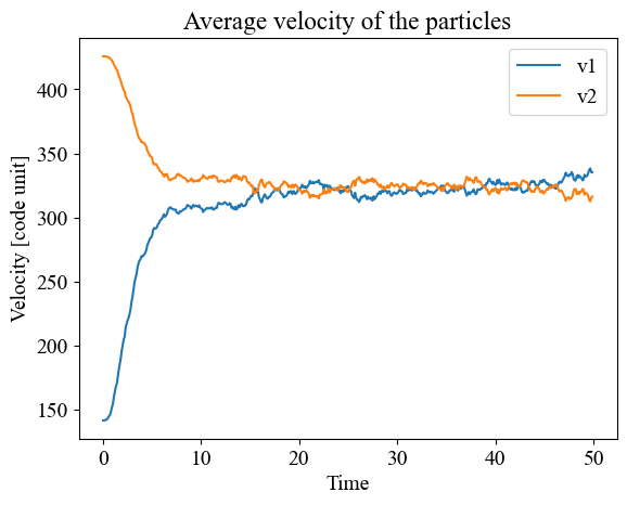
Figure 3: Mean velocities of two particle groups (v1, v2) approaching each other within ~15 time units
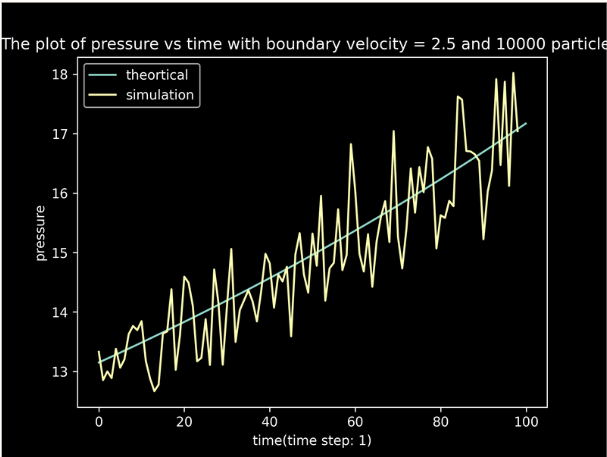
Figure 4: Moving-wall compression at boundary speed 2.5 code units — the closest agreement with theory among the speeds tested
Simulation Videos
Video 1: Mixing of two particle groups with different initial velocities — their mean velocities approach each other
Video 2: Adiabatic compression with a moving boundary (v=20) — particles accelerate as the boundary compresses the domain
2D N-Body Thermodynamics Simulation
Course
Computational Physics, NTHU
Period
Spring 2024
Overview
A group project for the NTHU Computational Physics course, using a 2D particle simulation to study ideal-gas behavior, moving-wall compression, and mixing of two particle populations. I built the main structure and first usable version of the simulation code. The final group project added pressure measurements, a spatial grid, inter-particle interactions, and comparisons with thermodynamic predictions.
- Personal contribution: Built the main structure and first usable version of the simulation code.
- Group implementation: Developed a 5×5 spatial partition, moving-wall boundary reflections, pressure output, RK2 time stepping, and collision and repulsive-force models.
- Group analysis: Compared simulated pressure with ideal-gas and adiabatic predictions, and examined particle trajectories, kinetic energy, and mixing.
Methodology
Spatial partition and interactions
The final code partitions the simulation box into a 5×5 grid. Its grid_N.py lookup restricts candidate interactions to nearby cells. Optional short-range repulsion and a simplified equal-mass collision rule are calculated in Numba-compiled loops. The code advances particle positions with an RK2 time-stepping routine.
Boundaries and pressure
The bound_reflection() routine updates four walls, reflects particles that cross them, and adjusts their normal velocity for wall motion. It estimates pressure from the particles' momentum changes over the time step and wall length. Moving one wall provides a compression experiment.
Comparisons
The final report compares simulated pressure with kinetic-theory and two-dimensional adiabatic predictions. It also plots particle trajectories, total kinetic energy, and the velocities of two populations with different initial conditions.
Results & Analysis
Ideal gas and compression
The group report found the general pressure trend but also a substantial discrepancy in the ideal-gas comparison. For moving-wall compression, the simulation agreed most closely with the theoretical curve at the slowest tested boundary speed, 2.5 code units; the deviation grew at higher speeds.
Particle interactions and mixing
The trajectory plots show how adding inter-particle collisions and repulsion changes particle paths. In the mixing experiment, total kinetic energy stayed approximately level, and the two groups' average-speed curves approached one another after about 15 time units.
Figures
Figure 1: Particle trajectories (0–25) with inter-particle collisions and short-range repulsion — showing their combined effect
Figure 2: Total kinetic energy vs time — the plotted value changes modestly during the run
Figure 3: Mean velocities of two particle groups (v1, v2) approaching each other within ~15 time units
Figure 4: Moving-wall compression at boundary speed 2.5 code units — the closest agreement with theory among the speeds tested
Simulation Videos
Video 1: Mixing of two particle groups with different initial velocities — their mean velocities approach each other
Video 2: Adiabatic compression with a moving boundary (v=20) — particles accelerate as the boundary compresses the domain