Modeling and Analysis of Kelvin–Helmholtz (KHI) and Rayleigh–Taylor (RTI) Instabilities
A group project comparing Kelvin–Helmholtz instability (KHI), driven by shear between fluid layers, and Rayleigh–Taylor instability (RTI), driven by a denser layer above a lighter one. We used two-dimensional Euler simulations with HLLC fluxes, varied density contrast and shear speed, and examined density and kinetic-energy images.
- ▪Group solver: Two-dimensional compressible Euler equations with HLLC fluxes in both directions. The provided RTI code uses Numba and a CFL-based time step on a 512×512 grid.
- ▪RTI runs: A smoothed density interface with a small cosine perturbation under gravity; displayed density-ratio cases include 3:1, 5:1, and 10:1.
- ▪KHI runs: Shear-layer simulations with varied velocity differences and density contrasts.
- ▪Outputs: Density snapshots, kinetic-energy maps, and simulation videos.
Methodology
Numerical method
The group used a two-dimensional compressible Euler solver with HLLC fluxes. The provided RTI implementation advances with a CFL-limited time step and uses Numba to compile its numerical loops.
Simulation setup
For RTI, a denser layer begins above a lighter layer. A smoothed interface and small cosine perturbation start the instability under gravity. For KHI, two layers move at different horizontal speeds. Runs vary density contrast and shear speed to compare the resulting structures.
Analysis
The project compares density snapshots, kinetic-energy maps, and videos across the parameter choices.
Results & Analysis
The RTI images show the heavy-fluid spike developing a wider head as it descends. Other density-ratio runs show changes in the shape of the spike and its edges. The KHI videos show the interface rolling into vortices under velocity shear. These are qualitative comparisons; the displayed images do not establish a measured growth rate.
Figures
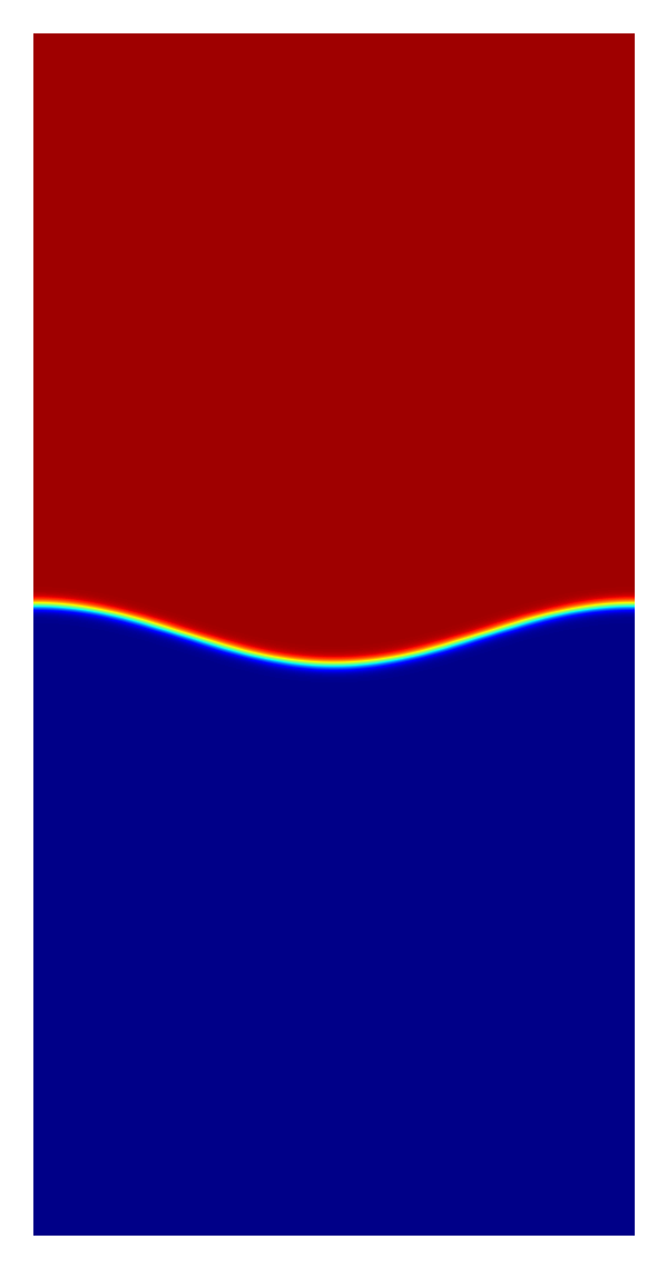
Figure 1: Initial RTI density field (3:1 density ratio, frame 0)
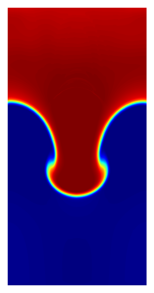
Figure 2: RTI density field (3:1 density ratio, frame 130)
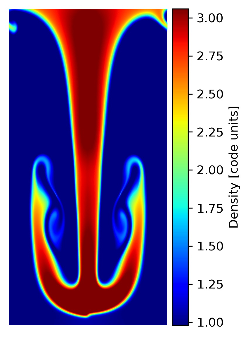
Figure 3: RTI density field (3:1 density ratio, frame 250)
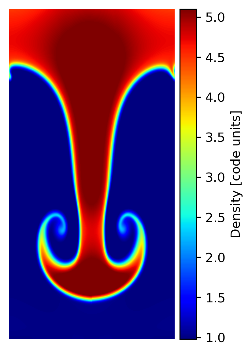
Figure 4: RTI density field (5:1 density ratio, frame 169)
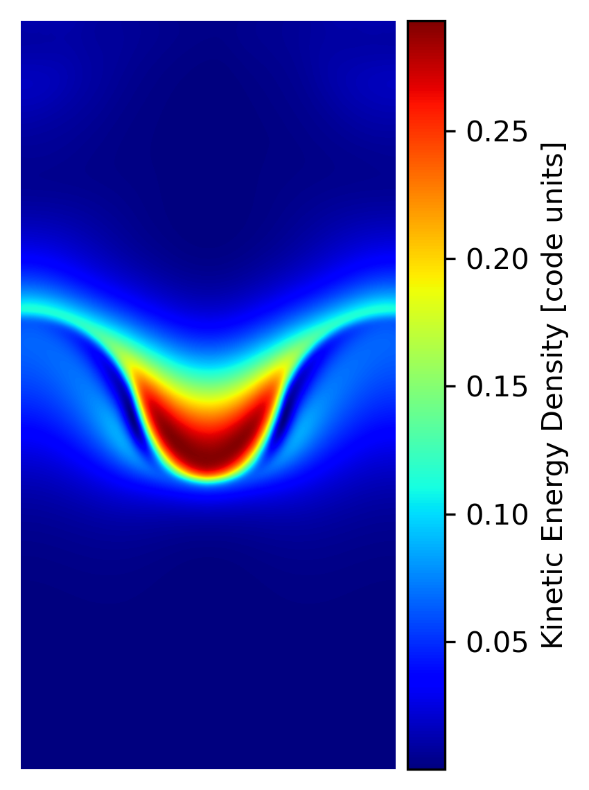
Figure 5: RTI kinetic-energy density (frame 100)
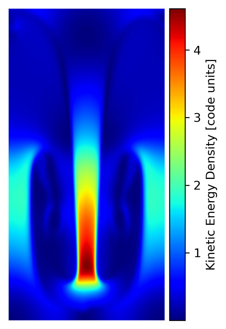
Figure 6: RTI kinetic-energy density (frame 250)
Simulation Videos
Video 1: RTI density-field evolution
Video 2: KHI density-field evolution (2.7:1 density ratio)
Video 3: KHI density-field evolution (shear speed difference 0.5 code units)
Modeling and Analysis of Kelvin–Helmholtz (KHI) and Rayleigh–Taylor (RTI) Instabilities
Course
Experimental Physics, NTHU
Period
Spring 2025
Overview
A group project comparing Kelvin–Helmholtz instability (KHI), driven by shear between fluid layers, and Rayleigh–Taylor instability (RTI), driven by a denser layer above a lighter one. We used two-dimensional Euler simulations with HLLC fluxes, varied density contrast and shear speed, and examined density and kinetic-energy images.
- Group solver: Two-dimensional compressible Euler equations with HLLC fluxes in both directions. The provided RTI code uses Numba and a CFL-based time step on a 512×512 grid.
- RTI runs: A smoothed density interface with a small cosine perturbation under gravity; displayed density-ratio cases include 3:1, 5:1, and 10:1.
- KHI runs: Shear-layer simulations with varied velocity differences and density contrasts.
- Outputs: Density snapshots, kinetic-energy maps, and simulation videos.
Methodology
Numerical method
The group used a two-dimensional compressible Euler solver with HLLC fluxes. The provided RTI implementation advances with a CFL-limited time step and uses Numba to compile its numerical loops.
Simulation setup
For RTI, a denser layer begins above a lighter layer. A smoothed interface and small cosine perturbation start the instability under gravity. For KHI, two layers move at different horizontal speeds. Runs vary density contrast and shear speed to compare the resulting structures.
Analysis
The project compares density snapshots, kinetic-energy maps, and videos across the parameter choices.
Results & Analysis
The RTI images show the heavy-fluid spike developing a wider head as it descends. Other density-ratio runs show changes in the shape of the spike and its edges. The KHI videos show the interface rolling into vortices under velocity shear. These are qualitative comparisons; the displayed images do not establish a measured growth rate.
Figures
Figure 1: Initial RTI density field (3:1 density ratio, frame 0)
Figure 2: RTI density field (3:1 density ratio, frame 130)
Figure 3: RTI density field (3:1 density ratio, frame 250)
Figure 4: RTI density field (5:1 density ratio, frame 169)
Figure 5: RTI kinetic-energy density (frame 100)
Figure 6: RTI kinetic-energy density (frame 250)
Simulation Videos
Video 1: RTI density-field evolution
Video 2: KHI density-field evolution (2.7:1 density ratio)
Video 3: KHI density-field evolution (shear speed difference 0.5 code units)